Postings on science, wine, and the mind, among other things.
Deep Learning the Big Five
Compressing personality via scoring, PCA, and autoencoder
People differ from one another in many ways. Some of these differences are momentary, like when one person feels happy and another feels sad. Other differences are more enduring. These can include physical differences, like height or eye color. They also include psychological differences, like whether a person tends to get angry easily, or whether they like to try new foods. Psychologists call these enduring psychological differences between people "traits." If you say that someone is bold, boorish, or brilliant, you are describing their traits.
Together, a person's traits form what we call their personality. Many psychologists are interested in describing the structure personality: how certain traits seem to be correlated with each other across people. For example, if you observe that someone is very punctual, you could make an educated guess that they also like to keep their house clean. Such a guess wouldn't always be right, but on average over many such guesses, you would be much more accurate than if you guessed randomly.
The most prominent modern theory of personality is the Five Factor Model, also known as the Big Five. The Big Five refers to five factors which describe most the correlations in traits between people. You can think of them a bit like the cardinal directions on a map: North vs. South, and East vs. West. Any other direction - like north-northwest - is some combination of these cardinal directions. In the same way, each trait can be thought of as a combination of the Big Five. The five factors are:
- Openness (to experience): Open people like to seek out new experiences, even if they may sometimes be risky.
- Conscientiousness: Conscientious people are disciplined and organized, but less spontaneous.
- Extraversion: Extraverted people love big social gatherings, whereas introverts tend to find such events taxing.
- Agreeableness: Agreeable people get along well with others, whereas disagree people tend to be more argumentative.
- Neuroticism: Neurotic people tend to experience more negative emotions and be more easily upset.
Readers unfamiliar with academic psychology may recognize some resemblance to the Myers-Briggs Type Indicator (MBTI). This taxonomy sorts people into one of 16 personality types based on 4 binary categories. Although the MBTI remains popular in corporate settings and dating apps, in scientific psychology it has long been superseded by theories like the Big Five, which are more reliable, valid, and comprehensive. These modern theories all feature continuous trait dimensions, rather than categories like the MBTI, because this is much more descriptive of the underlying reality (e.g., most people aren't radically introverted or extraverted, but rather somewhere in the middle). The Big Five isn't the only such modern theory of personality. It's best known competitor is the HEXACO model. However, HEXACO and Big Five are quite similar, with the main difference between them being HEXACO's extra "Honesty-Humility" factor. For simplicity, I will stick to the Big Five in this post.
The Big Five as a compression of personality
One way to think about a theory like the Big Five is as a compressed version of personality. It takes all of the related or synonymous traits - like friendly, affectionate, and helpful - and squeezes all the redundancy out of them, reducing hundreds of traits down to just the Big Five. In general, compression is very useful, because it makes something complicated and lengthy into something relatively short and simple. For example, we all benefit from compression every day as we look at images and watch videos on our phones and computers. There is a huge amount of redundancy in images: one pixel is very highly correlated with the one next to it. Similarly, in video one frame is very highly correlated with the next. Uncompressed image and video files are much larger, so using them would seriously affect our download times and data bills. For example, the jpg format commonly used to compress images reduces their size by a factor of 10, and the mpeg video format can make video files up to 200X smaller!
In terms of data size, the responses to a personality questionnaire are tiny: ~50 values on 5-point scales, versus millions of pixels in a single frame of 1080p video. Moreover, nearly everyone uses photos and videos, but relatively people few work with personality data. If compressing personality doesn't help us save space on our hard drives, why do researchers care about doing it? There are a few reasons:
- Interpretation: Try to visualize a 100-dimensional space. Not easy, eh? Computers are often perfectly happy to process high-dimensional spaces. Humans - or at least the parts of our brains involved in conscious, explicit reasoning - struggle with more then two or three dimensions. Compressing personality helps us to subjectively understand personality structure and talk about it with others.
- Generalization: Low-dimensional models typically generalize better than high dimensional models. For example, imagine you are trying to develop a model to explain the way that certain words tend to occur close to one another in a body of text. If you trained such a model on text from one place - let's say, reddit - you might get better performance out of a higher-dimensional model than a simpler model. However, if you applied those models to text from another source - like Twitter - you would likely find that the performance of the complex model degrades much more than that of the low-dimensional model, both proportionally and in absolute terms. In machine learning jargon, keeping your model simple helps prevent it from overfitting.
- Efficiency: If you find that people's personalities can be summarized quite well by just five numbers, you can construct a survey optimized to estimate those five numbers very efficiently. Rather than asking hundreds of random questions, you can target a few dozen to get the same result. This is practically useful, as it saves participants time and researchers money.
- Theory: The structure of personality is instrinsically interesting to personality psychologists. How many cardinal traits are there? What are they? Why do they emerge? Compressing personality answers, or makes it easier to answer, these sorts of questions.
Given that compression is desirable, how to do we achieve it? There are many different ways we could compress data, and some of them will be more efficient than others. For example, imagine the positions of the numbers on an analog clock. How could you efficiently represent those positions? Well, you could define an x-axis and a y-axis with an origin at the center of the clock. The position of each time could then be represented by its x- and y-coordinates. However, this approach fails to take advantage of the fact that the clock is circular. The distance from the center of the clock to each number is the same, so rather than being 2d, we could argue that the clock is actually a 1-d object on a 2-d plane. In this regime, the position of each point could be presented by a single number, indicating how far around the clocks it is (e.g., from 0 to 360 degrees). Representing the positions as cartesian points would require 24 numbers - 12 positions, 2 coordinates each. Representing them as a circle would require 13 numbers - one radius, plus 12 angular coordinates. This example illustrates how the way data is compressed can dramatically impact its ultimate size.
In practice, personality data are almost always compressed by a technique called factor analysis. Exploratory factor analysis (EFA) is typically used to get an initial sense for the structure of the data, and then confirmatory factor analysis (CFA) is used to validate this structure. EFA is quite similar to the more widely known dimensionality reduction technique of principal component analysis (PCA). There are some differences between EFA and PCA - particularly in how they deal with measurement error - but they are much more closely related to each other than either is to CFA.
After factor analysis has been used to discover and test the structure of some domain, it is common for researchers to develop a scale to efficiently measure that structure. For example, if you discover that there are five factors which explain most of personality, then you can put together a targeted set of questions which reflect where a person falls on each dimension. Scale construction is a complex engineering feat which often involves a lot more data collection and factor analysis. However, when it is done, it opens up another way to compress the data: scoring. Scoring simply means taking all of the questions which measure a particular trait, and adding up (or averaging) their ratings. This is so arithmetically simple that you could probably do it in your head. This is an appealingly simple way to compress personality, since in the old days (and occasionally still) personality questionnaires were scored by humans rather than computers. It also helps with interpretation, because typically the selected questions each reflect just one trait.
Comparing personality compression algorithms
As the clock analogy in the last section illustrates, the type of compression algorithm used can drastically influence the efficiency of compression, and the final structure of the compressed data. This makes it very important to consider how the way we compress personality data may be shaping the structure we attribute to personality. In this post, I will consider three different ways of compressing personality data: scoring the survey 'as intended', using PCA, and using deep learning in the form of a neural network called an autoencoder. I will apply each of these methods to ~1 million responses to the International Personality Item Pool's 50-question Big Five Factor Markers survey. The code for this blog post is available in juypter notebook form here.
Each method will compress the 50 responses made by each participant down to just five numbers. I will then use these five numbers to "reconstruct" each participant's original responses. Performance will be measured in terms of reconstruction error. That is, what is the difference between the actual ratings someone gives on the survey, and the ratings predicted based on each model's compressed 5-number representation. The smaller the reconstruction error, the less information is lost via compression, and thus the better the algorithm. I measured reconstruction error using root mean square error (RMSE). To ensure that the more powerful models don't get an unfair advantage due to overfitting, I split the data 90%-10%. The 90% was used to learn the PCA/autencoder parameters, and the performance of all three models was assessed in the independent 10%.
Baseline
I began by getting an initial baseline against which to compare the different compression algorithms. For this and all subsequent analyses, I put all items onto a 0-1 scale, instead of the original 1-5 scale. Note that some items were meant to be reverse scored (i.e., high ratings indicate lower factor scores), and those items were reversed accordingly. I scored the survey by averaging ratings from questions witin each of the five factors. I then averaged these ratings across participants to get the mean value for each of the five factors within the training set. I used these values to predict the ratings in the test set. In other words, I calculated the average extraversion across people, and used this average as the prediction for the ratings participants gave on each extraversion question. Guessing the mean personality is a pretty terrible way to make these predictions, but it's a good baseline, since it uses the simplest compression algorithm (scoring) and deliberately avoids using any information from the individual. No sensible compression of personality should do worse, but randomly guessing responses would.
The baseline calculation yields an RMSE of .305 - equivalent to making an average error of about 1.2 points on the original 5-point scale.
Scoring
Next, I scored the survey as described above, but *did not* average the scores across participants. Instead I used each participant's individual five-factor scores to predict the ratings on the questions associated with each factor. Note that this approach assumes that each question is an equally good indicator of the factor in question. This probably isn't a good assumption to make about questions in general, but the survey was engineered so that this works out pretty well with the specific questions it contains.
Compressing ratings via scoring yielded an RMSE of .235. This represent a big improvement over baseline, with error down ~23%.
PCA
PCA is a matrix factorization technique. It divides the data matrix into two new matrices which, when multiplied together, reproduce the original data matrix. However, whereas the columns of the data matrix might have been correlated with one another, the new ones are not. Moreover, the columns in the new matrices have been sorted by how much variance they explain in the original data matrix. We can thus throw away 45/50 of these columns to reduce the dimensionality of our data. In the process, we have lost relatively little information, because we kept the five columns which explained the most variance in the data. These five columns contain the weights telling us how to convert a participant's 50 responses down to just 5 numbers - the component scores. The model learnt these weights on the training data, and then applied them to compress the test data. I then used the same weights to reverse the process, generating unique predictions for each of the 50 questions. However, these predictions will be a bit off, because some information was inevitably lost in compression.
PCA differs from the scoring method in that it allows each question to contribute to each factor, rather averaging some questions for one factor, and other questions for another factor. PCA also differs from scoring in that the weights of each question can be different, so that if one question is a better indicator of a factor than others, it will get a higher weight. However, PCA and scoring are similar in that they are both linear methods. Effectively, they can only compress the data by taking some weighted average of the ratings.
Compressing ratings via PCA yielded a reconstruction RMSE of .215. This is better than the scoring method, but the difference between the two is only 29% of the difference between the scoring method and baseline. This makes sense, since the survey was constructed so that the assumptions made by scoring wouldn't be too far off.
Autoencoder
An autoencoder is a type of neural network which learns to optimally compress and then reconstruct data. The architecture of the autoencoder I used is illustrated in the image below. It features several dense (fully-connected) layers of 50 units each (in many autoencoders, these layers might get smaller over subsequent steps, but it doesn't make a huge difference). These are followed by a single hidden layer known as the "bottleneck" or "code" which contains only five units. This is the compressed representation of the personality data, with the same dimensionality (5) as that used in the scoring and PCA approaches. This is then followed by several more dense layers of size 50 which learn to "decompress" (i.e., reconstruct) the code back into the input.
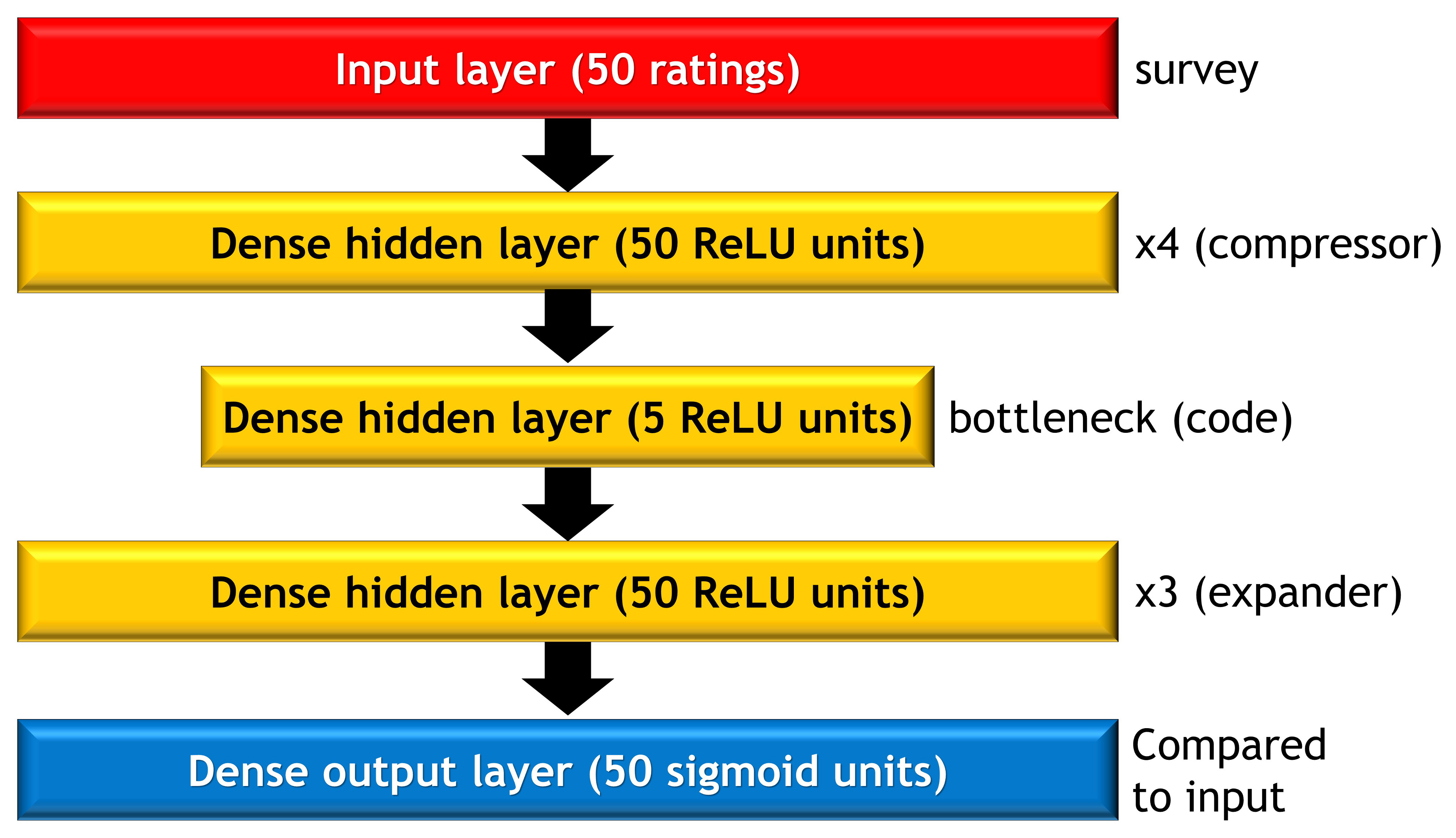
The compressor and decompressor portions of the network can learn fairly arbitrary nonlinear functions of the data. For example, they could learn what amount to interaction terms (in the more traditional psych jargon) such that they change the weighting of one question based on the response to another. The compressor could also learn to scale the responses to single items in a nonlinear way, such as treating both extremes as similar to each other, and the middle as different to both. Similarly, the decompressor network can also learn very complex nonlinear functions to take the compressed code and use it reconstruct the original input. This nonlinearity gives the autoencoder much greater power than the PCA to discover structure in the data and optimally (de)compress it. Often we might want to take measures to prevent this very compliated model from overfitting, such as using early stopping, dropout, or regularization. However, in this case we have a ton of data, and its relatively low dimensional, so overfitting is less of a worry. Indeed, the training and test set accuracy for this model end up being very similar. In any case, for the autoencoder to outperform the PCA, it needs some nonlinearity to find. If the system is linear, then the autoencoder should reach a conclusion similar to that of the PCA.
This is exactly what we find here: the autoencoder achieves an RMSE of .2096, only slightly better than that of the PCA approach. This improvement is only 25% of the already small improvement we see going from the scoring method to PCA, indicating that there is not much nonlinear structure to pick up on in this data.
Comparing scoring and autoencoder codes
As we've seen, PCA compresses personality only marginally better than scoring, and an autoencoder only marginally outperforms PCA. However, this does not necessarily mean that the autoencoder learned the same compression as the PCA or the scoring. In principle it's quite possible that the autoencoder learned some other representation of the data which bears little obvious resemblance to the Big Five. To test this, I compared the results of the scoring method to the autoencoder. Specifically, for each participant in the test set, I scored their survey, and also ran it through the autoencoder to extract the bottleneck layer activations. In half of the test set, I learned weights for a Procrustes transformation from the autoencoder code to the scores. This transformation rotates one set of variables to the orientation of another set, which is useful in this instance because the autoencoder might have been at any arbitrary orientation relative to the scoring. I applied this transformation to the activations in the left out half of the test set, so that there would be a 1-to-1 mapping of Big Five scores to autoencoder activations. Finally, I correlated the scores with the activations to see whether the autoencoder had learned the Big Five. You can see the results in the heatmap below.

As you can see, the autoencoder learns a representation very similar to that produced by simply scoring the survey. The correlation between hidden unit activity and scored factors ranged from r = .84-.95, and off-diagonal correlations were very small in comparison. This indicates that it was no coincidence that the different compression methods performed similarly: they had converged on similar compressed representations.
Nonlinear personality
As we have seen, using a deep neural network to compress personality yields similar results to simply scoring a survey in the intended manner. Should we take this as an indication that the structure of personality is primarily linear? The results don't contradict such a claim, but they do not provide much support for it either. The items in the Big Five survey do not represent a random sample from the population of possible questions you could ask about someone's behavior. Instead, they are a heavily curated list specifically designed to function well as a linear instrument. Any items with dramatically nonlinear response properties would likely have been culled in the survey generation process, because their nonlinearity would have lowered their (linear) correlation with other items. Thus, if the autoencoder had greatly outperformed the PCA on this data, this would have been very strong evidence for nonlinear structure in personality. The converse, however, is neither here nor there.
Examining a very large random selection of questions would be a better way to assess the presence of nonlinear structure in personality. However, asking participants 1000s of random questions isn't a terribly common practice for psychologists, for obvious reasons like cost and lack of utility. Indeed, merely trying to appropriately sample these questions from the hypothetical population of possible questions would be an interesting methodological challenge. Moreover, neural networks tend to need quite large samples to perform optimally, and it's hard to envisage a million people being eager to answer 1000s of random questions about themselves, rather than just 50 targeted questions with interpretable feedback.
However, there may be other, more practical ways to assess nonlinearity in personality. People are constantly using traits words to describe themselves and others in everyday life. Much of that everyday life now happens in public on the internet, where the text is available to anyone with the technical skills to retrieve it. How trait words are used in naturally occurring text may thus provide a more realistic avenue to revealing any interesting nonlinearities which dwell within our personalities.
© 2019 Mark Allen Thornton. All rights reserved.